Well Done!
Author: hazlina
BHE3232 – Digital System Design – Week 12 – Project
Submissions – Well Done!
- Dice Game Controller. Project Report

- Password Protected Digital Lock. Project Report

- v
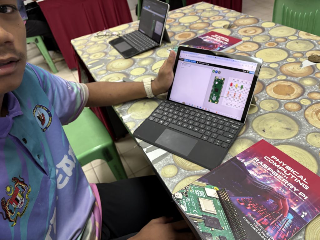
2025 Book :) Physical Computing with Raspberry Pi: A Hands-On Guide to Pico-Satellite Systems and Operations
The book is out 🙂
Raspberry Pi Programming 2025/3 – SMK Indera Shahbandar, Pekan
*UMPSA STEM Lab Raspberry Pi Programming Synopsis can be found here.
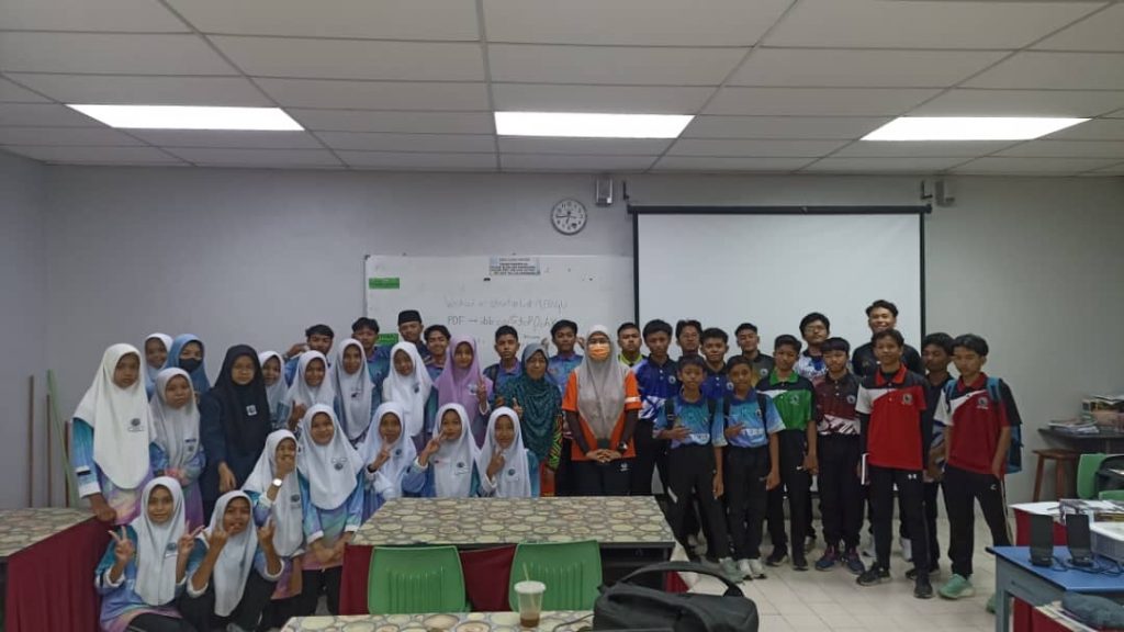
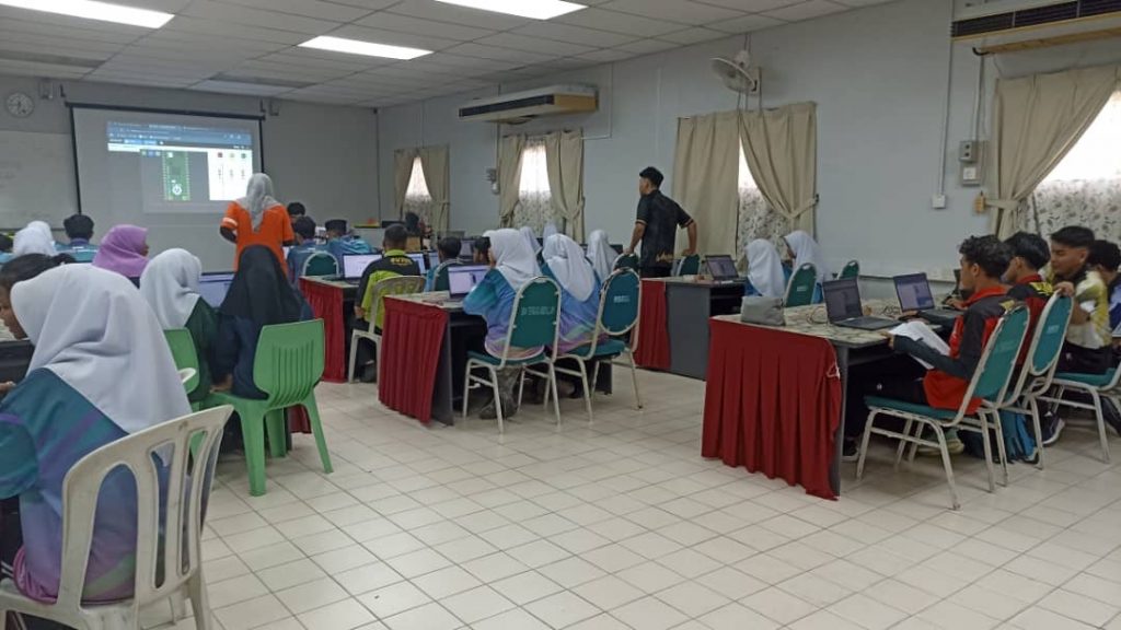
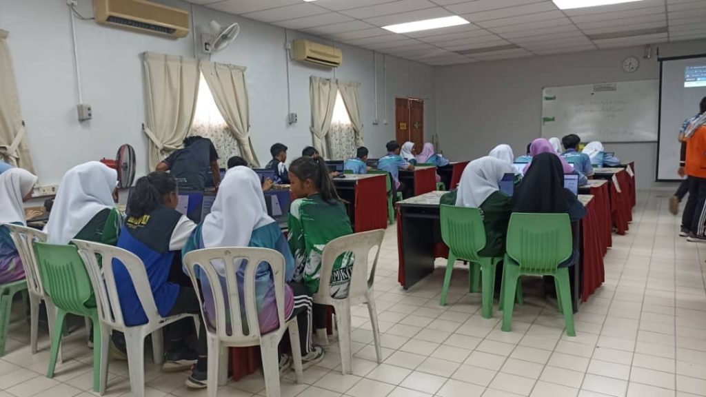
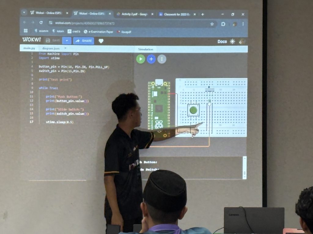
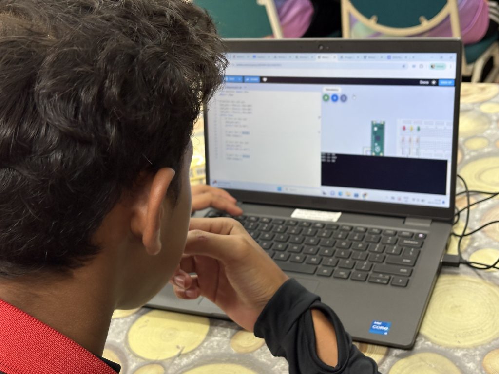
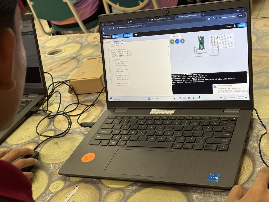
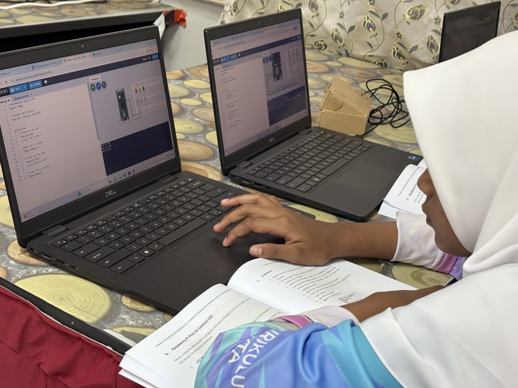
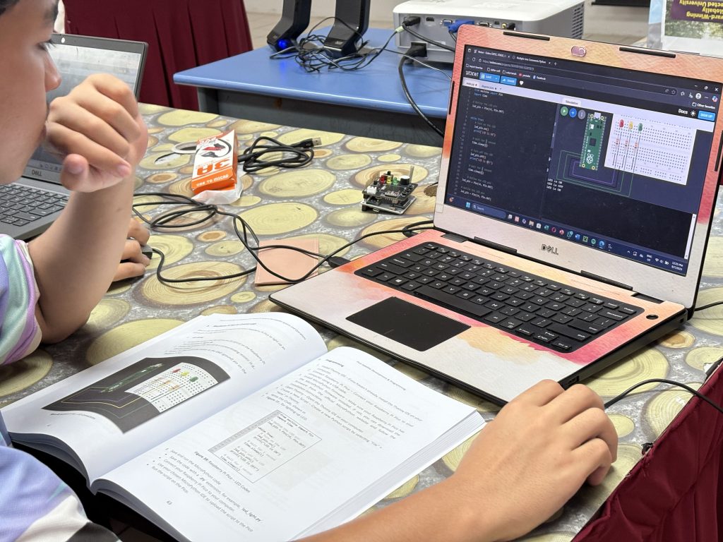
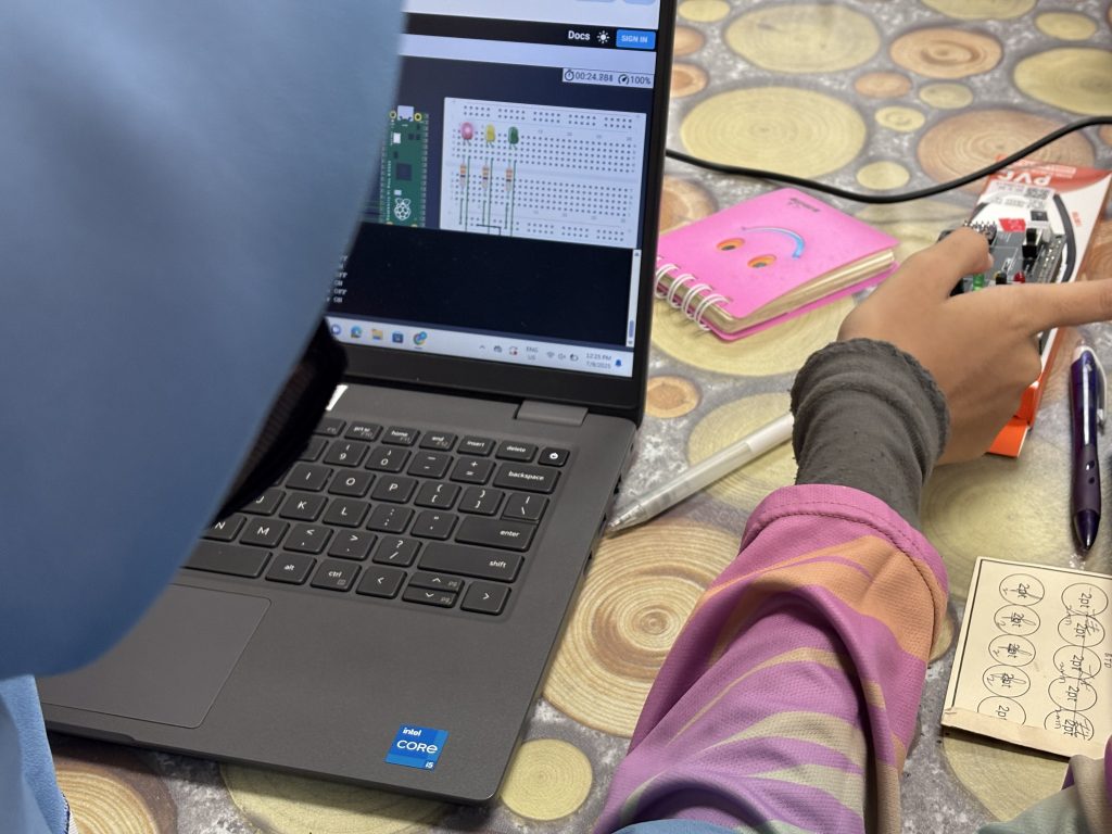
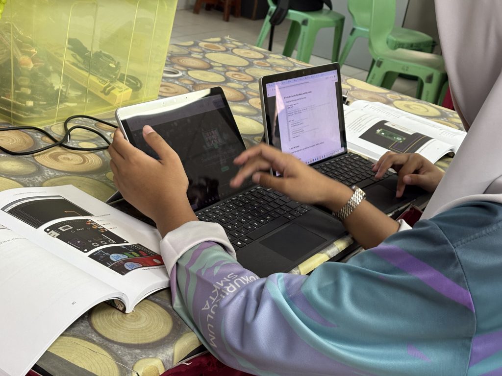
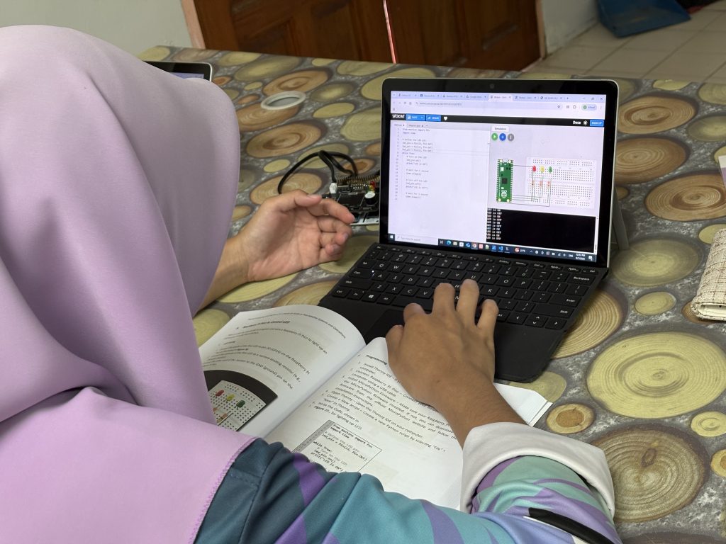
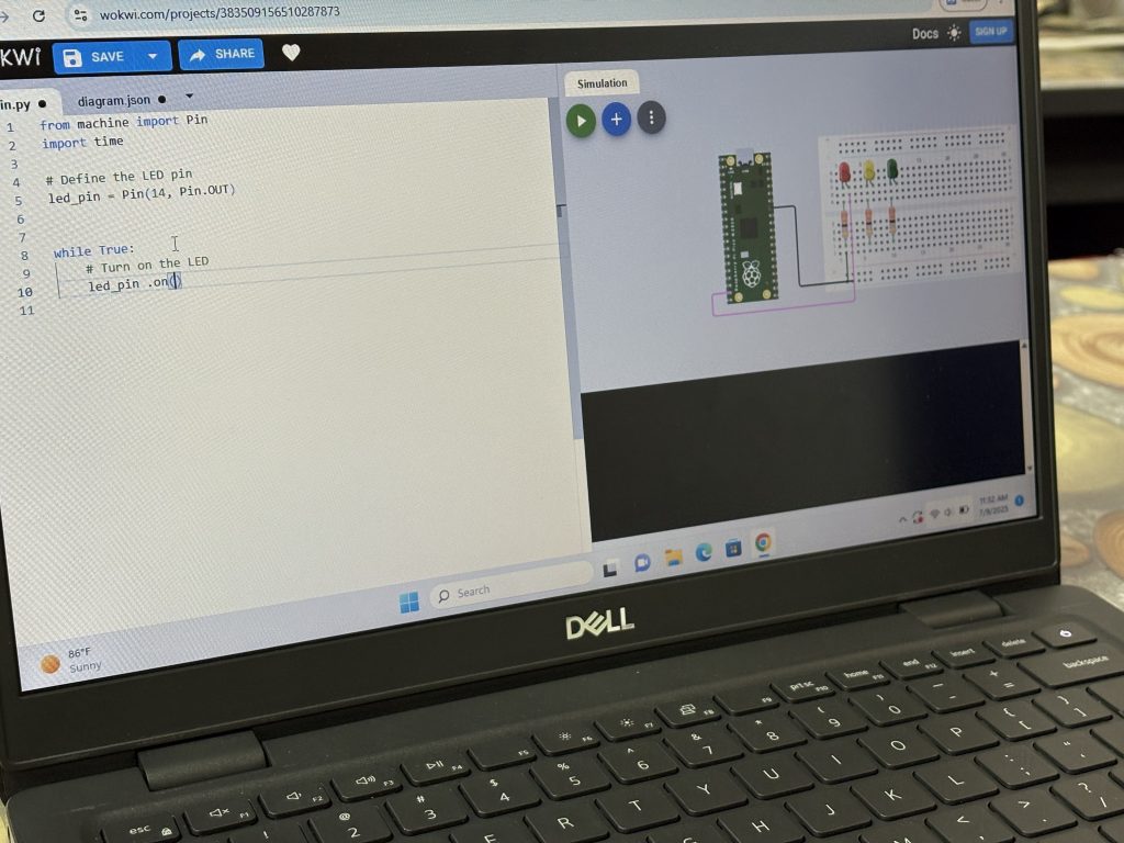
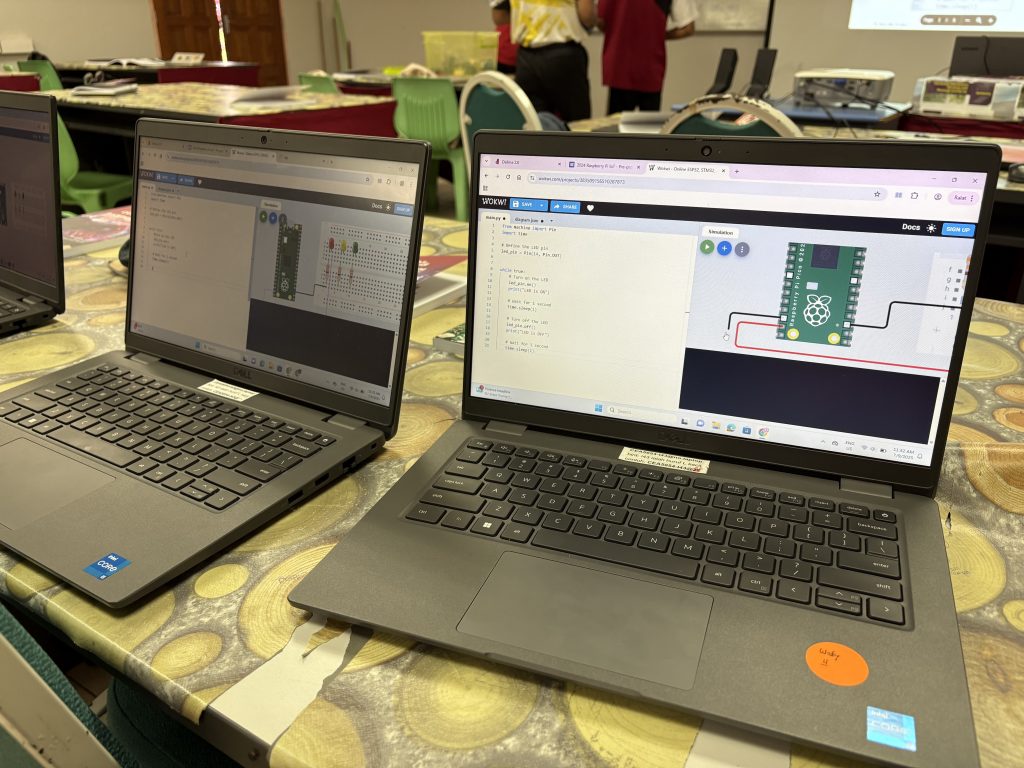
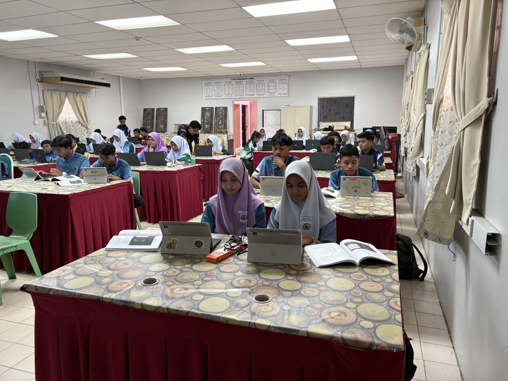
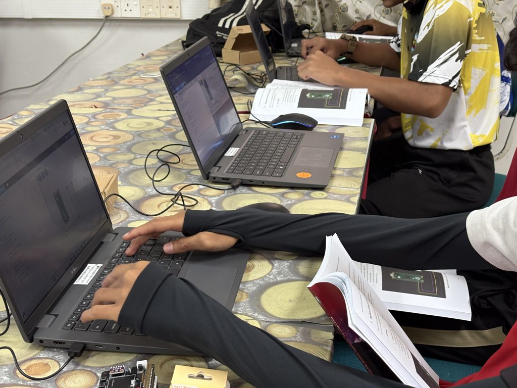
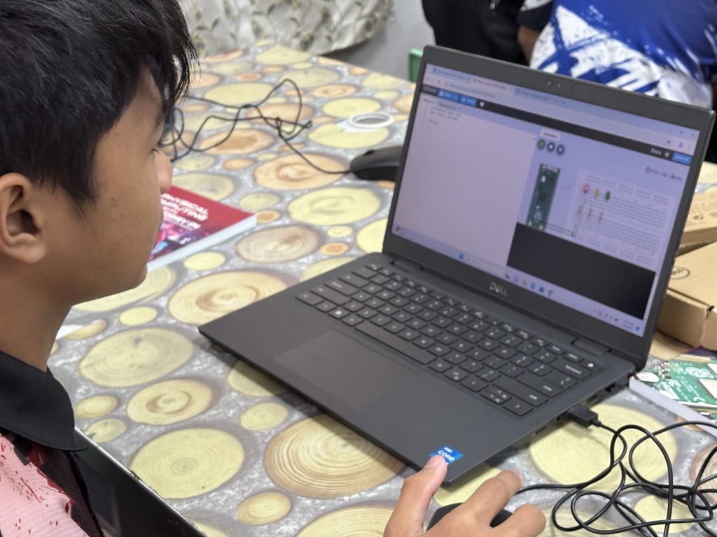
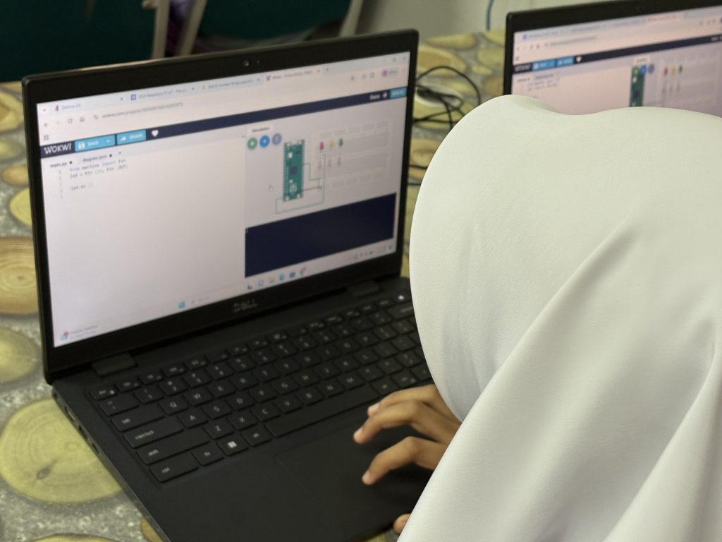
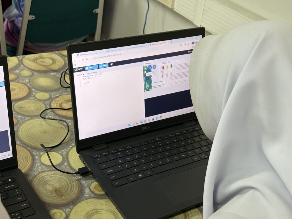
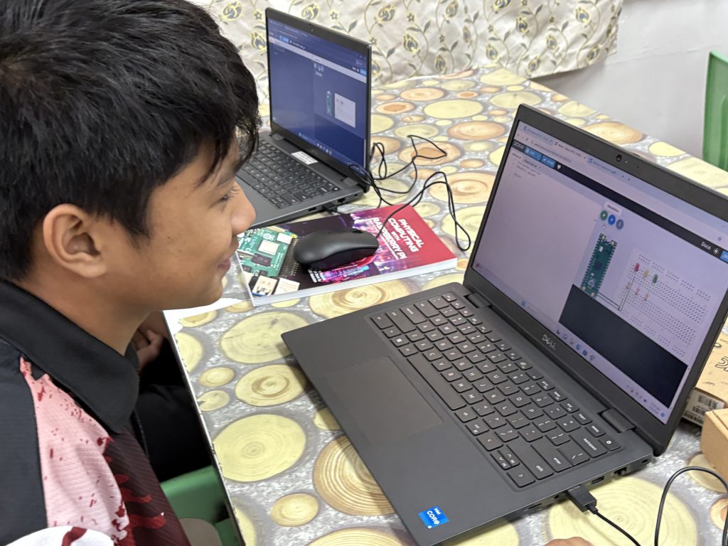
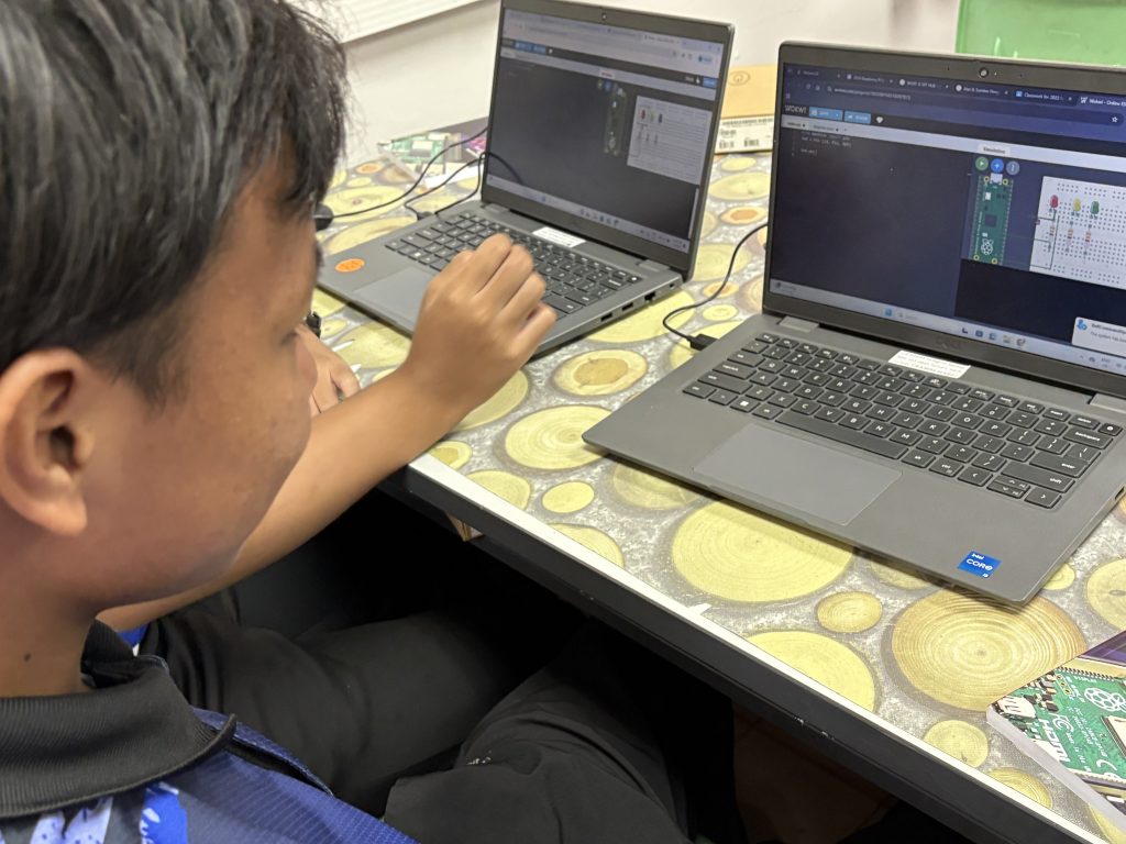
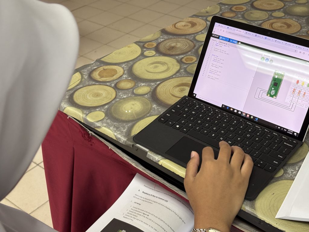
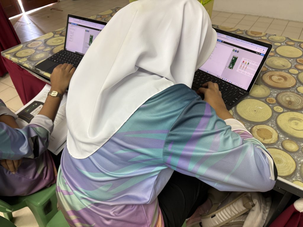
In the Raspberry Pi IoT session, 35 students and teachers from SMK Indera Shahbandar were introduced to the concept of the Internet of Things (IoT) using Raspberry Pi on the UMP STEM Cube, a pico-satellite learning kit specifically designed to facilitate engineering learning.
The content covered basic digital input/output operations on onboard LEDs, as well as topics such as dashboard design using gyro meter and BMU280 sensor data, including collecting and storing data in a cloud database. Participants learned to interface sensors with Raspberry Pi boards and develop IoT applications for real-world scenarios. The session provided students with valuable insights into IoT technology and its applications in various domains.
A special appreciation is extended to Cikgu Adzrul from SMK Indera Shahbandar for coordination in facilitating communication between the participants and the UMPSA STEM Lab :).
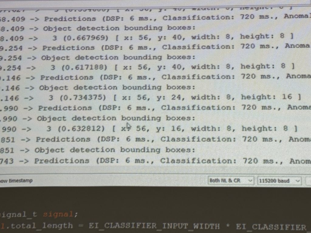
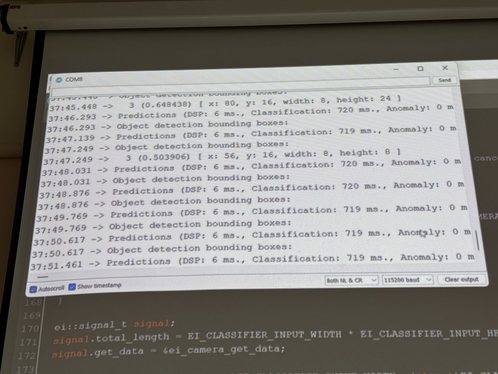
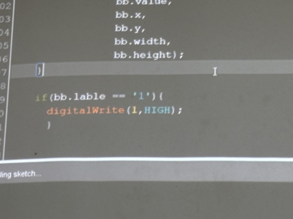
Module Development AI Chip

Discussion on FTIR Results


Discussion MDEC
Internship Evaluation 2024/25


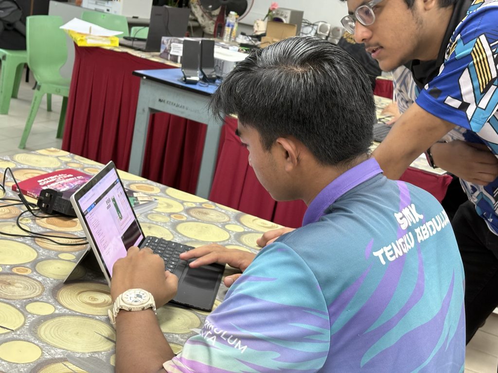
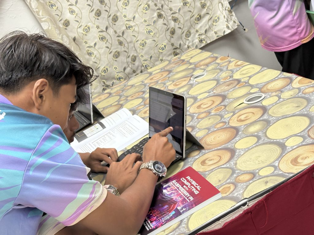
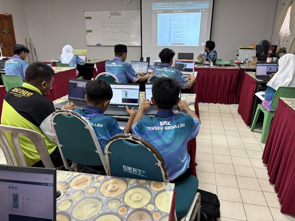
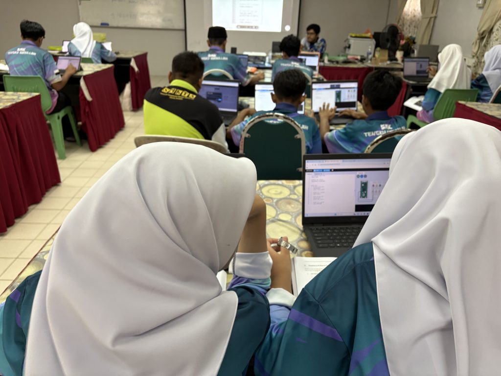
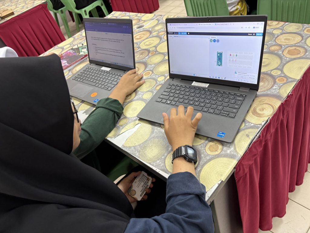
Raspberry Pi Programming 2025/2 – SMK Tuanku Abdullah Pekan
*UMPSA STEM Lab Raspberry Pi Programming Synopsis can be found here.
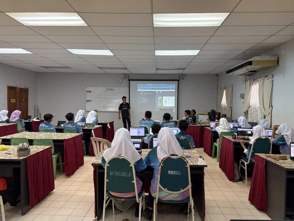
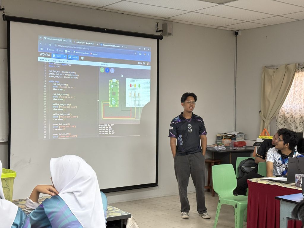
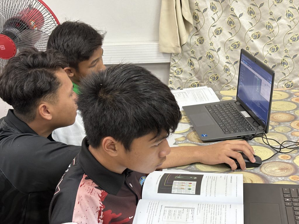
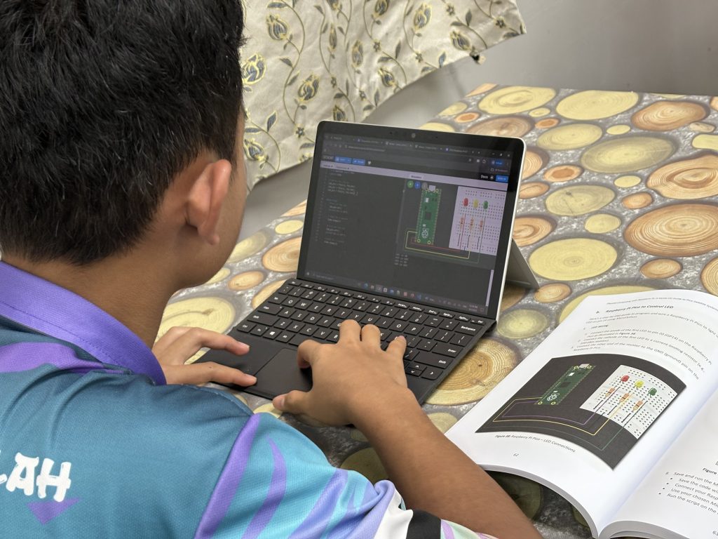
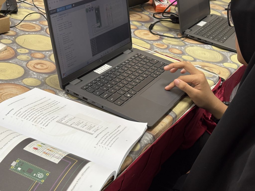
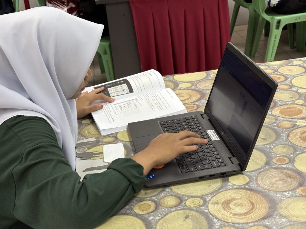
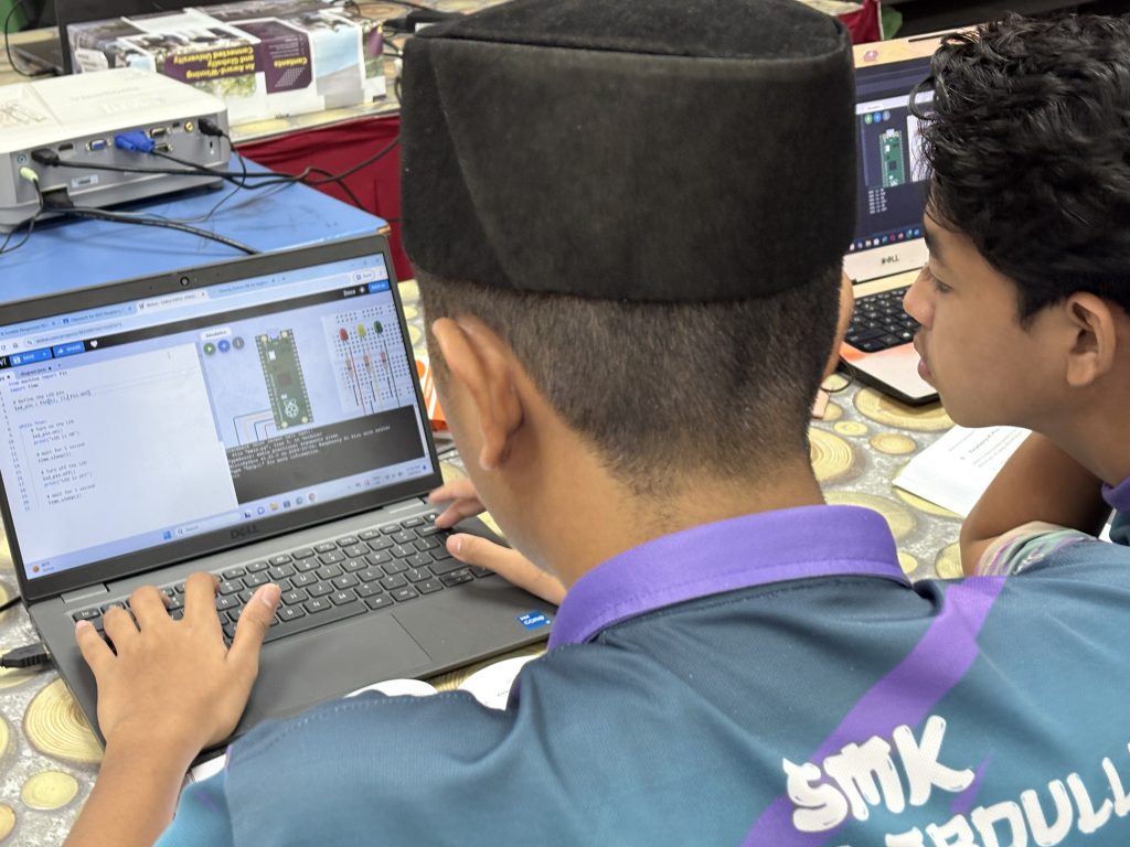
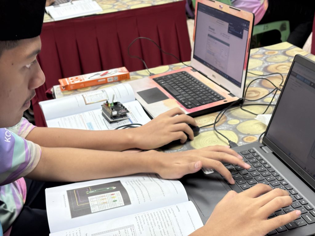
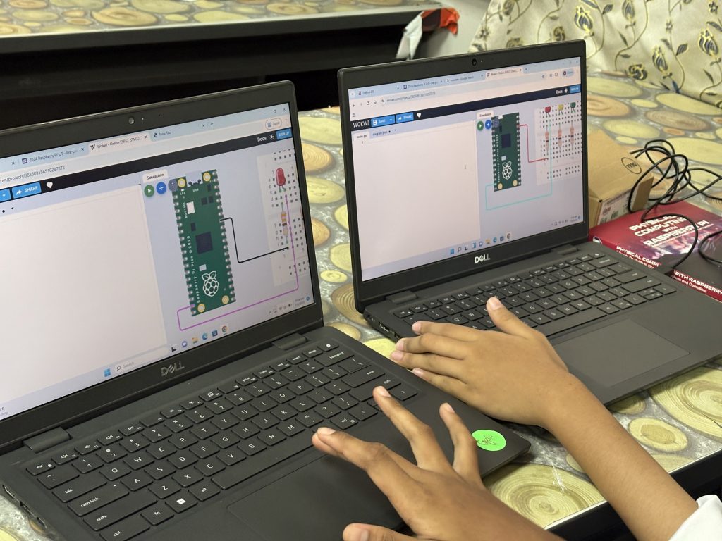
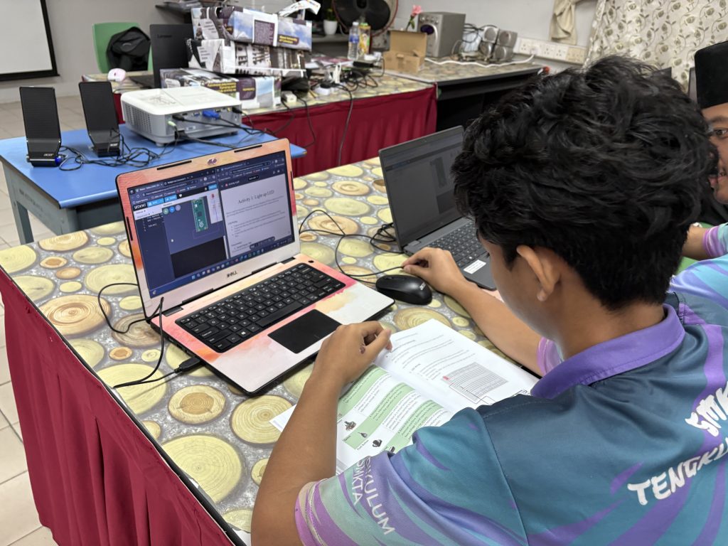
In the Raspberry Pi IoT session, 60 students and teachers from SMK Tuanku Abdullah were introduced to the concept of the Internet of Things (IoT) using Raspberry Pi on the UMP STEM Cube, a pico-satellite learning kit specifically designed to facilitate engineering learning.
The content covered basic digital input/output operations on onboard LEDs, as well as topics such as dashboard design using gyro meter and BMU280 sensor data, including collecting and storing data in a cloud database. Participants learned to interface sensors with Raspberry Pi boards and develop IoT applications for real-world scenarios. The session provided students with valuable insights into IoT technology and its applications in various domains.
A special appreciation is extended to Cikgu Zulkarnain and Cikgu Zaiti from SMK TA for coordination in facilitating communication between the participants and the UMPSA STEM Lab :).


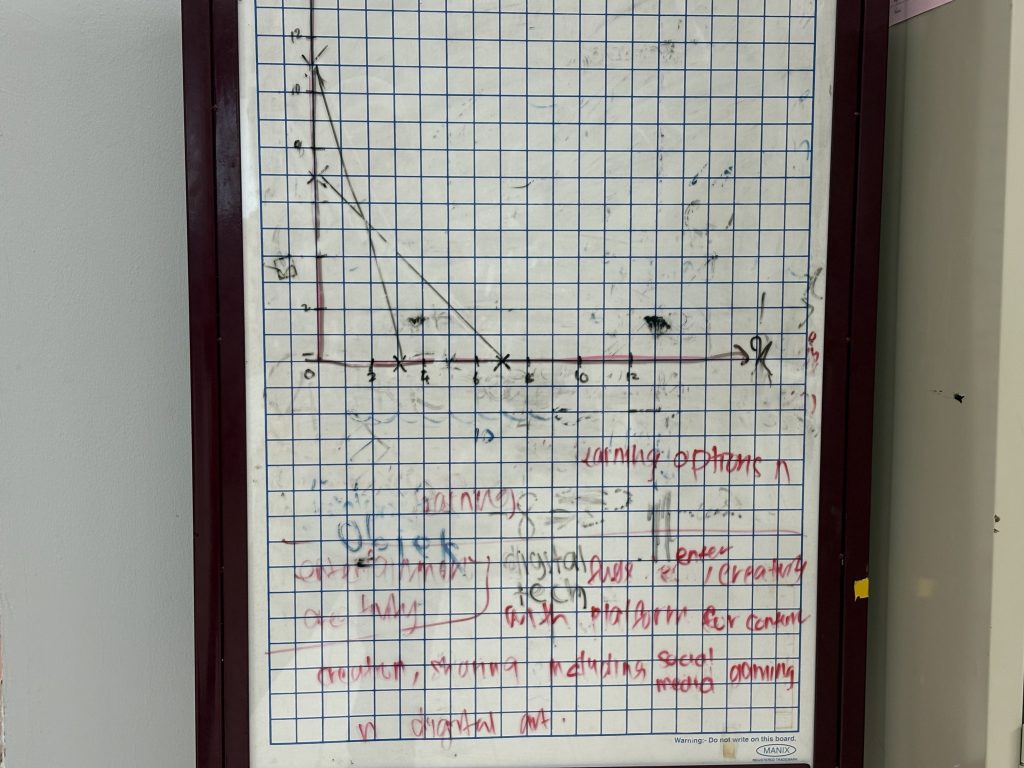
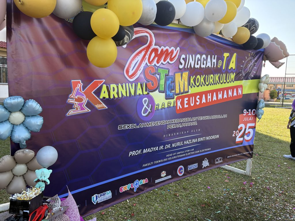
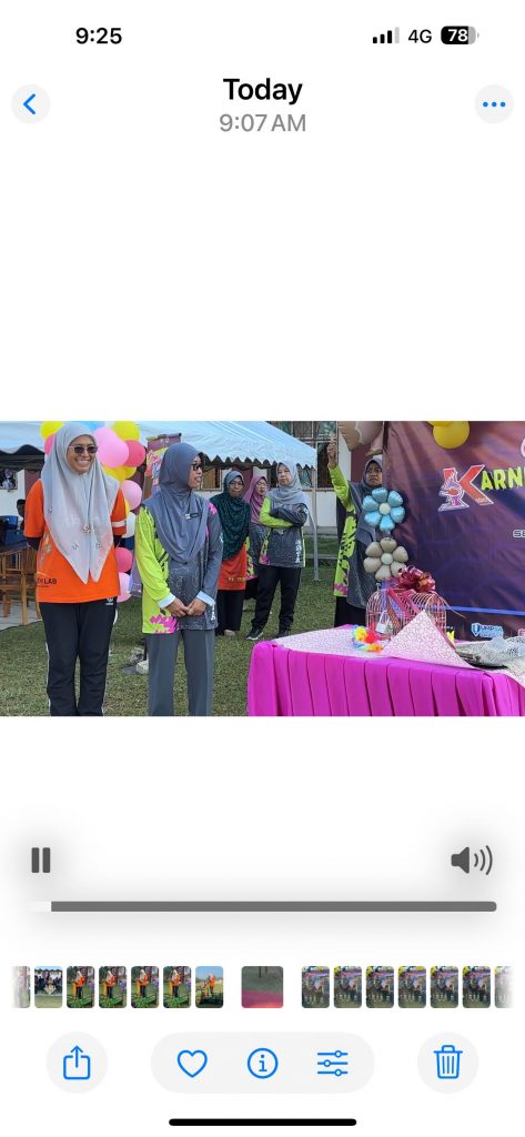
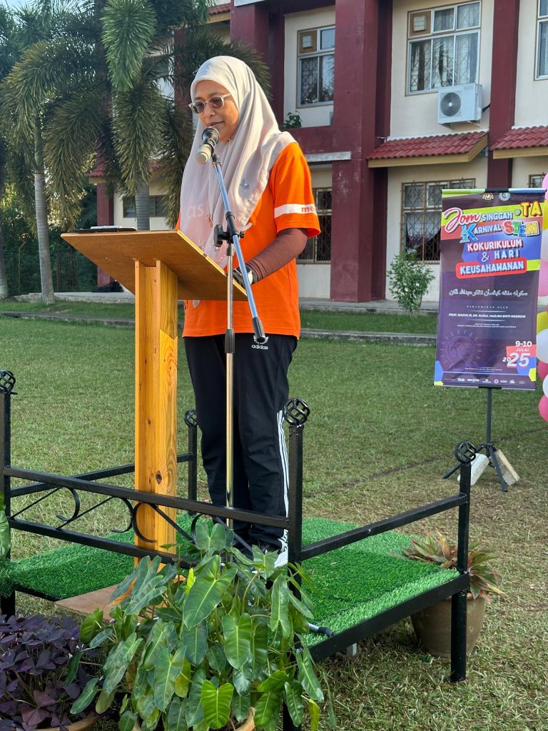
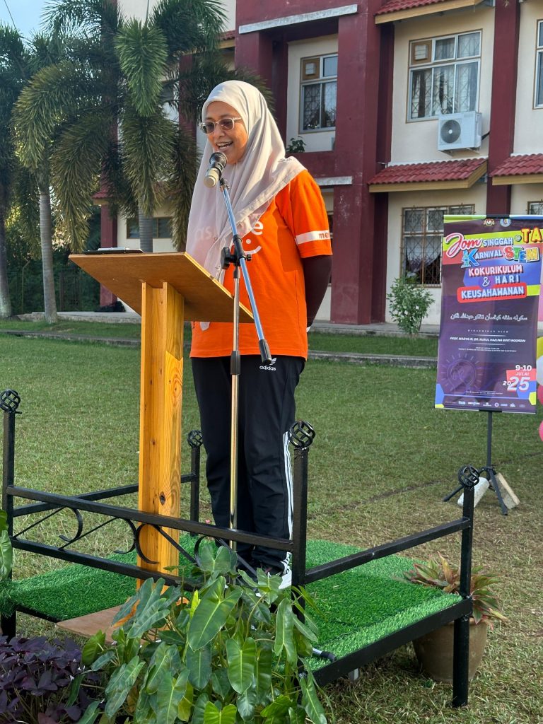
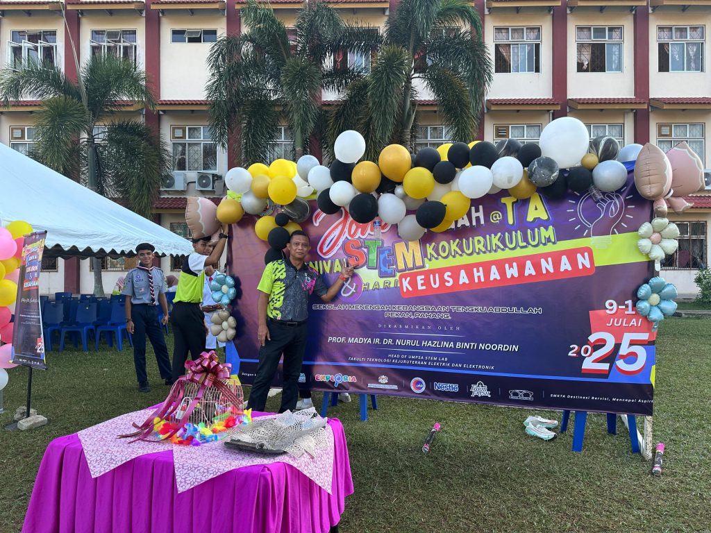
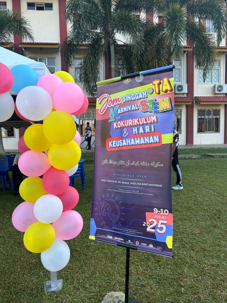
STEM – Co-curriculum – Entrepreneurship
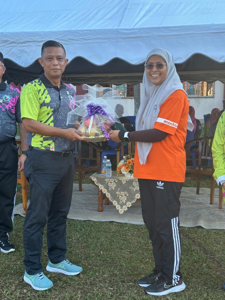
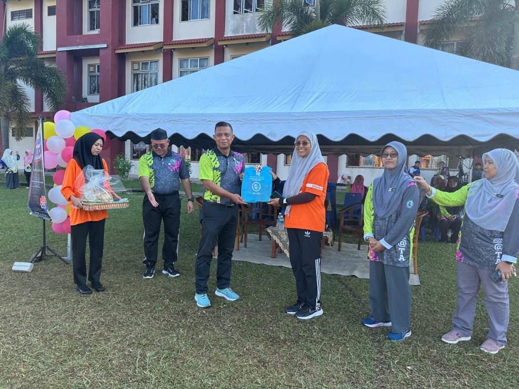
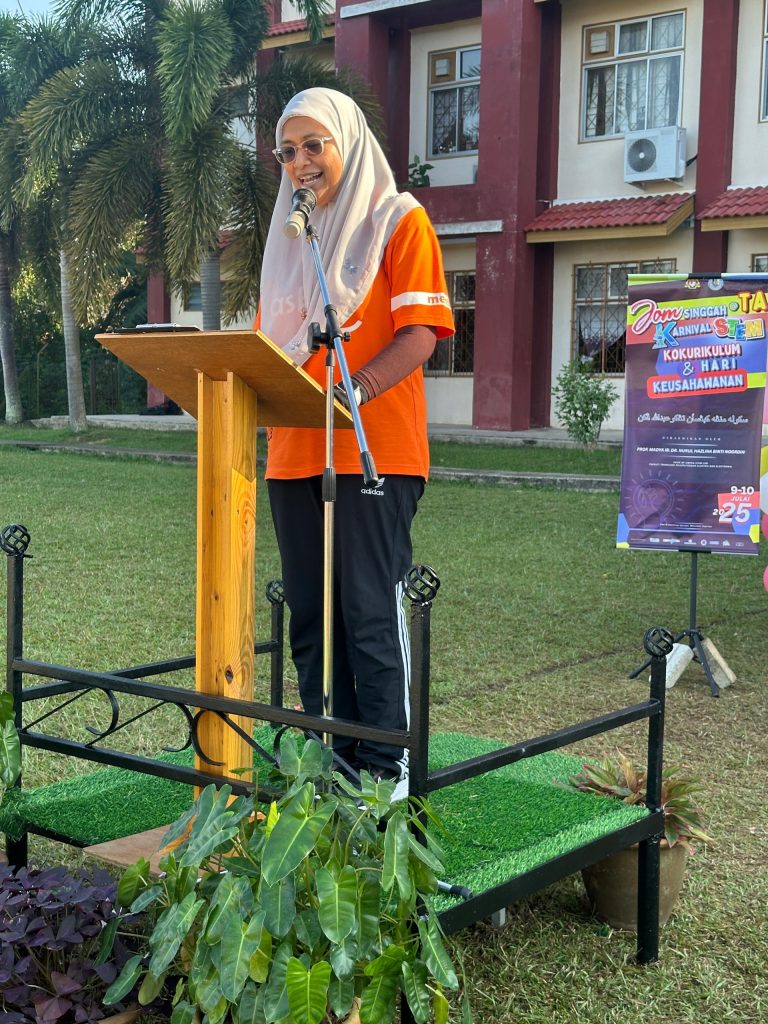
Today, I had the honour of being invited to officiate the launch of the STEM-CO Curriculum-Entrepreneurship Program at SMK Tuanku Abdullah. The event was more than just a launch — it was a meaningful milestone in how we approach STEM education, entrepreneurship, and student empowerment.
The STEM-CO (STEM + Co-curriculum + Entrepreneurship) framework is a forward-thinking initiative designed to integrate STEM learning with real-world entrepreneurial experiences. At its core, this curriculum encourages students to go beyond textbooks, empowering them to identify opportunities (or simply said as “menghidu peluang keusahawanan”), solve community problems, and develop STEM-based innovations with commercial potential.
What makes this program exciting is its interconnectedness. STEM teaches students to think critically and solve problems. Entrepreneurship teaches them to act on those ideas and create value. Together, they form a powerful ecosystem that cultivates STEM leadership — nurturing a generation of thinkers, doers, and changemakers.
Throughout the event, I was inspired by the energy and vision of the students and teachers. Their enthusiasm reaffirmed my belief that when students are given the right platforms and guidance, they can thrive as future technopreneurs and leaders of innovation.
Kudos to SMK Tuanku Abdullah and all stakeholders for championing this initiative. May this be the spark that ignites many more innovations to come.